GPU-accelerated simulation using MuJoCo Warp¶

So far, we have been simulating a single fly at a time on the CPU. This is sufficient for many tasks, but some applications—such as training a neural network controller through reinforcement learning, exploring the effect of a parameter over a large population of model variants, or replaying a large bulk of experimental data—require running hundreds or thousands of simulations simultaneously.

This is where the GPU shines. While a CPU has a small number of powerful cores optimized for sequential execution, a GPU has thousands of simpler cores that can all run simultaneously. Rather than computing the next physics state for 1000 flies one after another, a GPU can update all 1000 flies at the same time.

FlyGym uses MuJoCo Warp to bring this capability to fly simulation. MuJoCo Warp is a GPU port of MuJoCo built on top of NVIDIA Warp, a Python framework for writing high-performance GPU kernels. The FlyGym GPUSimulation class wraps MuJoCo Warp to provide the same interface you already know from Simulation, while running all worlds in parallel on the GPU.

In this tutorial we will:

1. Run a basic batch simulation with 100 and then 1000 parallel worlds.
2. Enable GPU-side batch rendering so that all worlds are rendered on the GPU simultaneously.
3. Write custom GPU kernels in Warp to feed control inputs directly on the GPU, avoiding costly CPU–GPU data transfers and unlocking maximum throughput.

Before we start, let's confirm that a compatible GPU is available:

In [1]:

from flygym.warp.utils import check_gpu

check_gpu()

from flygym.warp.utils import check_gpu check_gpu()

Warp 1.12.0 initialized:
   CUDA Toolkit 12.9, Driver 13.0
   Devices:
     "cpu"      : "x86_64"
     "cuda:0"   : "NVIDIA GeForce RTX 3080 Ti" (12 GiB, sm_86, mempool enabled)
   Kernel cache:
     /home/sibwang/.cache/warp/1.12.0

Basic GPU simulation¶

As in Tutorial 2: Replaying experimental recordings and inferring dynamical quantities, we start by creating a fly spawned into an empty world:

In [2]:

from flygym.compose import Fly, ActuatorType, FlatGroundWorld, KinematicPosePreset
from flygym.anatomy import Skeleton, JointPreset, ActuatedDOFPreset, AxisOrder
from flygym.utils.math import Rotation3D


def make_model(
    joints_preset=JointPreset.LEGS_ONLY,
    actuated_dofs_preset=ActuatedDOFPreset.LEGS_ACTIVE_ONLY,
    actuator_type=ActuatorType.POSITION,
    position_gain=50.0,
    neutral_pose=KinematicPosePreset.NEUTRAL,
    spawn_position=(0, 0, 0.8),  # xyz in mm
    spawn_rotation=Rotation3D("quat", (1, 0, 0, 0)),
):

    fly = Fly()
    axis_order = AxisOrder.YAW_PITCH_ROLL

    # Add joints
    skeleton = Skeleton(axis_order=axis_order, joint_preset=joints_preset)
    fly.add_joints(skeleton, neutral_pose=neutral_pose)

    # Add position actuators and set them to the neutral pose
    actuated_dofs_list = fly.skeleton.get_actuated_dofs_from_preset(
        actuated_dofs_preset
    )
    fly.add_actuators(
        actuated_dofs_list,
        actuator_type=actuator_type,
        kp=position_gain,
        neutral_input=neutral_pose,
    )

    # Add leg adhesion
    fly.add_leg_adhesion()

    # Add visuals
    fly.colorize()
    cam = fly.add_tracking_camera()

    # Create a world and spawn the fly
    world = FlatGroundWorld()
    world.add_fly(fly, spawn_position, spawn_rotation)
    
    return fly, world, cam


fly, world, cam = make_model()

from flygym.compose import Fly, ActuatorType, FlatGroundWorld, KinematicPosePreset from flygym.anatomy import Skeleton, JointPreset, ActuatedDOFPreset, AxisOrder from flygym.utils.math import Rotation3D def make_model( joints_preset=JointPreset.LEGS_ONLY, actuated_dofs_preset=ActuatedDOFPreset.LEGS_ACTIVE_ONLY, actuator_type=ActuatorType.POSITION, position_gain=50.0, neutral_pose=KinematicPosePreset.NEUTRAL, spawn_position=(0, 0, 0.8), # xyz in mm spawn_rotation=Rotation3D("quat", (1, 0, 0, 0)), ): fly = Fly() axis_order = AxisOrder.YAW_PITCH_ROLL # Add joints skeleton = Skeleton(axis_order=axis_order, joint_preset=joints_preset) fly.add_joints(skeleton, neutral_pose=neutral_pose) # Add position actuators and set them to the neutral pose actuated_dofs_list = fly.skeleton.get_actuated_dofs_from_preset( actuated_dofs_preset ) fly.add_actuators( actuated_dofs_list, actuator_type=actuator_type, kp=position_gain, neutral_input=neutral_pose, ) # Add leg adhesion fly.add_leg_adhesion() # Add visuals fly.colorize() cam = fly.add_tracking_camera() # Create a world and spawn the fly world = FlatGroundWorld() world.add_fly(fly, spawn_position, spawn_rotation) return fly, world, cam fly, world, cam = make_model()

Now we are ready to create a simulation instance. Unlike previous tutorials, here we will use the GPUSimulation class from the warp module of FlyGym. The key difference is that we can specify how many worlds we want to simulate in parallel.

Note that all worlds must share the same model. They can run different data (i.e., different control inputs, leading to different fly trajectories), but the models themselves must be identical (i.e., flies in all worlds must have the same joint properties, body geometry, and so on).

In [3]:

from flygym.warp import GPUSimulation

n_worlds = 100

sim = GPUSimulation(world, n_worlds)

from flygym.warp import GPUSimulation n_worlds = 100 sim = GPUSimulation(world, n_worlds)

/home/sibwang/Projects/flygym/src/flygym/warp/simulation.py:411: UserWarning: MJWarp does not support noslip iterations. Changing option/noslip_iterations from 5 to 0.
  warnings.warn(

As before, we can attach a renderer to the simulation object. The difference here is that we can specify which worlds to render. If the worlds argument is left unspecified, all worlds will be rendered. This, however, might not be desirable because they may consume an enormous amount of memory, depending on how many worlds you are simulating in parallel. Here we will render the first 9 worlds.

In [4]:

renderer = sim.set_renderer(
    cam,
    playback_speed=0.2,
    output_fps=25,
    worlds=list(range(9)),  # render the first 9 worlds only
)

renderer = sim.set_renderer( cam, playback_speed=0.2, output_fps=25, worlds=list(range(9)), # render the first 9 worlds only )

As in Tutorial 2: Replaying experimental recordings and inferring dynamical quantities, we now load some experimentally recorded kinematic data.

In [5]:

from flygym_demo.spotlight_data import MotionSnippet

snippet = MotionSnippet()
sim_timestep = 1e-4

dof_angles = snippet.get_joint_angles(
    output_timestep=sim_timestep,
    output_dof_order=fly.get_actuated_jointdofs_order(ActuatorType.POSITION),
)
# dof_angles shape: (n_total_steps, n_dofs) — smoothed, interpolated, reordered
print(f"Total steps available: {dof_angles.shape[0]}, n_dofs: {dof_angles.shape[1]}")

from flygym_demo.spotlight_data import MotionSnippet snippet = MotionSnippet() sim_timestep = 1e-4 dof_angles = snippet.get_joint_angles( output_timestep=sim_timestep, output_dof_order=fly.get_actuated_jointdofs_order(ActuatorType.POSITION), ) # dof_angles shape: (n_total_steps, n_dofs) — smoothed, interpolated, reordered print(f"Total steps available: {dof_angles.shape[0]}, n_dofs: {dof_angles.shape[1]}")

Total steps available: 20000, n_dofs: 42

Since GPUs achieve their efficiency through parallelization, it is often desirable to break the computing task into small chunks that can be distributed over many GPU threads. For demonstration, we split the kinematic recording into 0.1 s snippets. Each world would get a different snippet (although for any practical application, 0.1 s is probably too short). When all possible 1 s chunks are exhausted, remaining worlds will get repeated copies.

In [6]:

import numpy as np

sim_seconds = 0.1
sim_steps = int(sim_seconds / sim_timestep)


def make_target_angles_all_worlds(n_worlds, sim_steps=sim_steps):
    """Prepare the input array for all worlds.
    World 0 gets 0s-0.1s, world 1 gets 0.1s-0.2s, etc.
    """
    n_total_steps, n_dofs = dof_angles.shape
    dof_angles_all_worlds = np.zeros((n_worlds, sim_steps, n_dofs), dtype=np.float32)
    n_partitions = n_total_steps // sim_steps
    for world_id in range(n_worlds):
        partition_idx = world_id % n_partitions
        start_idx = partition_idx * sim_steps
        end_idx = start_idx + sim_steps
        dof_angles_all_worlds[world_id] = dof_angles[start_idx:end_idx]
    return dof_angles_all_worlds


dof_angles_all_worlds = make_target_angles_all_worlds(n_worlds)

import numpy as np sim_seconds = 0.1 sim_steps = int(sim_seconds / sim_timestep) def make_target_angles_all_worlds(n_worlds, sim_steps=sim_steps): """Prepare the input array for all worlds. World 0 gets 0s-0.1s, world 1 gets 0.1s-0.2s, etc. """ n_total_steps, n_dofs = dof_angles.shape dof_angles_all_worlds = np.zeros((n_worlds, sim_steps, n_dofs), dtype=np.float32) n_partitions = n_total_steps // sim_steps for world_id in range(n_worlds): partition_idx = world_id % n_partitions start_idx = partition_idx * sim_steps end_idx = start_idx + sim_steps dof_angles_all_worlds[world_id] = dof_angles[start_idx:end_idx] return dof_angles_all_worlds dof_angles_all_worlds = make_target_angles_all_worlds(n_worlds)

We can now implement the main simulation loop. Again, this is very similar to the CPU-based simulation loop in Tutorial 2. The key difference here is that the set_leg_adhesion_states and set_actuator_inputs methods require inputs for all worlds. In other words, there is an additional world dimension in the input arrays. This also applies to other methods such as get_joint_angles.

In [7]:

from tqdm import trange  # for progress bar

fly_name = fly.name

sim.reset()

# Turn adhesion on for all 6 legs across all worlds
sim.set_leg_adhesion_states(fly_name, np.ones((n_worlds, 6), dtype=np.float32))

# As before, warm up the simulation for a few steps before applying the control inputs
sim.warmup()

# Run simulation loop
for step in trange(sim_steps):
    control_inputs = dof_angles_all_worlds[:, step, :]
    sim.set_actuator_inputs(fly_name, ActuatorType.POSITION, control_inputs)
    sim.step_with_profile()
    sim.render_as_needed_with_profile()

from tqdm import trange # for progress bar fly_name = fly.name sim.reset() # Turn adhesion on for all 6 legs across all worlds sim.set_leg_adhesion_states(fly_name, np.ones((n_worlds, 6), dtype=np.float32)) # As before, warm up the simulation for a few steps before applying the control inputs sim.warmup() # Run simulation loop for step in trange(sim_steps): control_inputs = dof_angles_all_worlds[:, step, :] sim.set_actuator_inputs(fly_name, ActuatorType.POSITION, control_inputs) sim.step_with_profile() sim.render_as_needed_with_profile()

Module flygym.warp.utils 37edc43 load on device 'cuda:0' took 0.90 ms  (cached)
Module mujoco_warp._src.smooth f756680 load on device 'cuda:0' took 8.85 ms  (cached)
Module mujoco_warp._src.collision_driver 4d8b905 load on device 'cuda:0' took 0.75 ms  (cached)
Module _nxn_broadphase__locals__kernel_83765485 8376548 load on device 'cuda:0' took 0.99 ms  (cached)
Module _primitive_narrowphase__locals__primitive_narrowphase_91741e55 91741e5 load on device 'cuda:0' took 0.66 ms  (cached)
Module mujoco_warp._src.constraint 63c97cb load on device 'cuda:0' took 3.52 ms  (cached)
Module mujoco_warp._src.sensor 912ac95 load on device 'cuda:0' took 3.13 ms  (cached)
Module mujoco_warp._src.forward 7114b3d load on device 'cuda:0' took 1.72 ms  (cached)
Module mujoco_warp._src.passive 7fb8524 load on device 'cuda:0' took 1.41 ms  (cached)
Module mul_m_sparse__locals___mul_m_sparse_47846b9f 47846b9 load on device 'cuda:0' took 1.01 ms  (cached)
Module _energy_vel_kinetic__locals__energy_vel_kinetic_59655b93 dfb3ea0 load on device 'cuda:0' took 1.04 ms  (cached)
Module mujoco_warp._src.forward 5a5c0b5 load on device 'cuda:0' took 1.65 ms  (cached)
Module mujoco_warp._src.support 343d1ae load on device 'cuda:0' took 1.10 ms  (cached)
Module mujoco_warp._src.solver eaac975 load on device 'cuda:0' took 2.51 ms  (cached)
Module solve_init_jaref__locals__kernel_329403b2 329403b load on device 'cuda:0' took 1.03 ms  (cached)
Module mul_m_sparse__locals___mul_m_sparse_dad9b434 dad9b43 load on device 'cuda:0' took 0.89 ms  (cached)
Module update_constraint_efc__locals__kernel_d4ac54f8 d4ac54f load on device 'cuda:0' took 0.83 ms  (cached)
Module update_constraint_gauss_cost__locals__kernel_ecc98ff8 ecc98ff load on device 'cuda:0' took 0.84 ms  (cached)
Module update_gradient_JTDAJ_sparse_tiled__locals__kernel_cf788183 0386d79 load on device 'cuda:0' took 1.27 ms  (cached)
Module update_gradient_cholesky_blocked__locals__kernel_24528e03 35eb900 load on device 'cuda:0' took 167.05 ms  (cached)
Module linesearch_jv_fused__locals__kernel_b3e1d056 b3e1d05 load on device 'cuda:0' took 9.41 ms  (cached)
Module linesearch_iterative__locals__kernel_8563129c 43c49b2 load on device 'cuda:0' took 1.26 ms  (cached)
Module update_constraint_efc__locals__kernel_5c3dedb8 5c3dedb load on device 'cuda:0' took 0.99 ms  (cached)
Module _contact_sort__locals__contact_sort_34f0bb85 1079711 load on device 'cuda:0' took 0.86 ms  (cached)

100%|██████████| 1000/1000 [00:06<00:00, 146.11it/s]

As in Tutorial 2, we call sim.step_with_profile() and sim.render_as_needed_with_profile to time code execution behind the scenes. This allows us to use sim.print_performance_report() to see a breakdown of compute time shown below. In practice, you can replace these with sim.step() and sim.render_as_needed(), which ironically should be a bit faster because we remove the timing overhead.

In [8]:

sim.print_performance_report()

sim.print_performance_report()

PERFORMANCE PROFILE

Stage	Time/step (us)	Percent (%)	Throughput (iters/s)	Throughput x realtime	Throughput (iters/s) (parallelized)	Throughput x realtime (parallelized)
Physics simulation advancement	5527	82	181	0.02	18094	1.81
Rendering*	1197	18	836	0.08	7522	0.75
TOTAL	6723	100	149	0.01	14874	1.49

* Note: 13 frames were rendered out of 1000 steps. Therefore, rendering time per image is 92039 us.

You might have observed two things from the two code blocks above: first, the simulation actually took much longer to run than the CPU version in Tutorial 2. Second, it took a long time before the actual simulation—indicated by the progress bar—started, and a bunch of log messages about GPU-side initialization got printed.

The answer to the first question is that we have to remember that we are running 100 worlds in parallel! Therefore, the overall execution speed is 100x faster. (You might notice that even so, this speed is still not very impressive. We will get to faster stuff later on in this tutorial.)

The answer to the second question is that GPU code needs to be compiled first. Therefore, the first time you simulate every model (and the first time only), it's going to take a bit longer.

---

As before, we can display the rendered videos. We will display the nine worlds that we rendered on a grid. This can be done simply by passing a list of world IDs to the show_in_notebook method (or save_video). If a single integer world ID is given, only that one world will be displayed or saved.

The scale argument control the factor by which each video is downscaled: for example, with 0.5, the width and height of each video is reduced by half. This prevents excessive memory usage when many worlds are rendered. If scale is unspecified, the videos will be scaled down so that the overall video has roughly the size of a single camera—this is likely too small though.

In [9]:

renderer.show_in_notebook(world_id=list(range(9)), scale=0.5)

renderer.show_in_notebook(world_id=list(range(9)), scale=0.5)

world [0, 1, 2, 3, 4, 5, 6, 7, 8], camera nmf/trackcam

Instead of 100 worlds, what if we simulate 1000 worlds in parallel?

Let's first consolidate the code in the few blocks above into a run_simulation function. In order to make sure that different simulations do not influence each other unexpectedly, we will create the model and generate the target angles from scratch for every simulation. Keep this in mind for the rest of this tutorial: every time we run a simulation, ~2-3 seconds are spent regenerating the model and the data, which is unnecessary for most practical use cases so the overhead is actually smaller.

In [10]:

def run_simulation(n_worlds):
    dof_angles_all_worlds = make_target_angles_all_worlds(n_worlds)
    
    fly, world, cam = make_model()
    fly_name = fly.name
    
    sim = GPUSimulation(world, n_worlds)
    renderer = sim.set_renderer(
        cam,
        playback_speed=0.2,
        output_fps=25,
        worlds=list(range(9)),  # render the first 9 worlds only
    )
    
    sim.set_leg_adhesion_states(fly_name, np.ones((n_worlds, 6), dtype=np.float32))
    sim.warmup()
    for step in trange(sim_steps):
        control_inputs = dof_angles_all_worlds[:, step, :]
        sim.set_actuator_inputs(fly_name, ActuatorType.POSITION, control_inputs)
        sim.step_with_profile()
        sim.render_as_needed_with_profile()
    
    sim.print_performance_report()
    renderer.show_in_notebook(world_id=list(range(9)), scale=0.5)

def run_simulation(n_worlds): dof_angles_all_worlds = make_target_angles_all_worlds(n_worlds) fly, world, cam = make_model() fly_name = fly.name sim = GPUSimulation(world, n_worlds) renderer = sim.set_renderer( cam, playback_speed=0.2, output_fps=25, worlds=list(range(9)), # render the first 9 worlds only ) sim.set_leg_adhesion_states(fly_name, np.ones((n_worlds, 6), dtype=np.float32)) sim.warmup() for step in trange(sim_steps): control_inputs = dof_angles_all_worlds[:, step, :] sim.set_actuator_inputs(fly_name, ActuatorType.POSITION, control_inputs) sim.step_with_profile() sim.render_as_needed_with_profile() sim.print_performance_report() renderer.show_in_notebook(world_id=list(range(9)), scale=0.5)

We can now simulate 1000 worlds at once (still rendering only 9).

In [11]:

run_simulation(n_worlds=1000)

run_simulation(n_worlds=1000)

/home/sibwang/Projects/flygym/src/flygym/warp/simulation.py:411: UserWarning: MJWarp does not support noslip iterations. Changing option/noslip_iterations from 5 to 0.
  warnings.warn(
100%|██████████| 1000/1000 [00:18<00:00, 53.70it/s]

PERFORMANCE PROFILE

Stage	Time/step (us)	Percent (%)	Throughput (iters/s)	Throughput x realtime	Throughput (iters/s) (parallelized)	Throughput x realtime (parallelized)
Physics simulation advancement	8099	44	123	0.01	123471	12.35
Rendering*	10236	56	98	0.01	879	0.09
TOTAL	18335	100	55	0.01	54539	5.45

* Note: 13 frames were rendered out of 1000 steps. Therefore, rendering time per image is 787415 us.

world [0, 1, 2, 3, 4, 5, 6, 7, 8], camera nmf/trackcam

Did the simulation take 10× longer? No! The time spent on physics simulation remained largely constant when going from 100 to 1000 worlds.

This is the core advantage of GPU simulation: as long as the total number of parallel worlds stays within the hardware's capacity, the GPU can handle additional worlds for little additional cost, because idle cores simply pick up the extra work. Depending on the GPU and the complexity of the simulation model, this "free scaling" region can extend from a few hundred to tens of thousands of parallel worlds before the hardware becomes saturated and throughput begins to degrade.

GPU-side batch rendering¶

Despite now simulating 1000 worlds at once, we are still rendering only 9 of them. This is becasue rendering each world takes quite a bit of time. Just as how we simulated all 1000 worlds in parallel, can we also do the rendering in parallel on the GPU?

The answer is yes: GPU-side rendering is supported by MuJoCo Warp and Warp itself. To use this, we need to toggle the use_gpu_batch_rendering to True.

In [12]:

def run_simulation_with_batch_rendering(n_worlds):
    dof_angles_all_worlds = make_target_angles_all_worlds(n_worlds)
    
    fly, world, cam = make_model()
    fly_name = fly.name
    
    sim = GPUSimulation(world, n_worlds)
    renderer = sim.set_renderer(
        cam,
        playback_speed=0.2,
        output_fps=25,
        use_gpu_batch_rendering=True,  # enable GPU batch rendering
        worlds=None,  # None: by default, all worlds are rendered
    )
    
    sim.set_leg_adhesion_states(fly_name, np.ones((n_worlds, 6), dtype=np.float32))
    sim.warmup()
    for step in trange(sim_steps):
        control_inputs = dof_angles_all_worlds[:, step, :]
        sim.set_actuator_inputs(fly_name, ActuatorType.POSITION, control_inputs)
        sim.step_with_profile()
        sim.render_as_needed_with_profile()
    
    sim.print_performance_report()
    # still only display the first 9 worlds in the notebook
    renderer.show_in_notebook(world_id=list(range(9)), scale=0.5)

def run_simulation_with_batch_rendering(n_worlds): dof_angles_all_worlds = make_target_angles_all_worlds(n_worlds) fly, world, cam = make_model() fly_name = fly.name sim = GPUSimulation(world, n_worlds) renderer = sim.set_renderer( cam, playback_speed=0.2, output_fps=25, use_gpu_batch_rendering=True, # enable GPU batch rendering worlds=None, # None: by default, all worlds are rendered ) sim.set_leg_adhesion_states(fly_name, np.ones((n_worlds, 6), dtype=np.float32)) sim.warmup() for step in trange(sim_steps): control_inputs = dof_angles_all_worlds[:, step, :] sim.set_actuator_inputs(fly_name, ActuatorType.POSITION, control_inputs) sim.step_with_profile() sim.render_as_needed_with_profile() sim.print_performance_report() # still only display the first 9 worlds in the notebook renderer.show_in_notebook(world_id=list(range(9)), scale=0.5)

In [13]:

run_simulation_with_batch_rendering(n_worlds=100)

run_simulation_with_batch_rendering(n_worlds=100)

/home/sibwang/Projects/flygym/src/flygym/warp/rendering.py:422: UserWarning: Adding overhead light for body nmf/c_thorax
  warnings.warn(f"Adding overhead light for body {body.full_identifier}")
/home/sibwang/Projects/flygym/src/flygym/warp/simulation.py:293: UserWarning: The world was modified to be compatible with GPU batch rendering. Recompiling the model.
  warnings.warn(

Module mujoco_warp._src.render_util 9cda0d9 load on device 'cuda:0' took 9.66 ms  (cached)
Module mujoco_warp._src.io 959c1b4 load on device 'cuda:0' took 3.39 ms  (cached)
Module mujoco_warp._src.bvh bd340bf load on device 'cuda:0' took 1.34 ms  (cached)

  3%|▎         | 26/1000 [00:00<00:07, 133.43it/s]

Module render__locals___render_megakernel_34319075 3431907 load on device 'cuda:0' took 10.14 ms  (cached)

100%|██████████| 1000/1000 [00:06<00:00, 155.42it/s]

PERFORMANCE PROFILE

Stage	Time/step (us)	Percent (%)	Throughput (iters/s)	Throughput x realtime	Throughput (iters/s) (parallelized)	Throughput x realtime (parallelized)
Physics simulation advancement	6080	96	164	0.02	16446	1.64
Rendering*	227	4	4409	0.44	440901	44.09
TOTAL	6307	100	159	0.02	15855	1.59

* Note: 13 frames were rendered out of 1000 steps. Therefore, rendering time per image is 17447 us.
Module map_mul 57ac4f6 load on device 'cuda:0' took 9.01 ms  (cached)

world [0, 1, 2, 3, 4, 5, 6, 7, 8], camera nmf/trackcam

Note that the appearance of the rendered scene is a bit different. For example, for memory efficiency, we have disabled texture rendering on the fly. The lighting also differs.

On the brighter side, the amount of time spent on rendering has significantly reduced. Don't forget that we are also rendering 1000 worlds now, not just 9, even though we have only displayed the first 9.

Running the whole simulation loop on the GPU¶

So far, the simulation loop still runs on the CPU: at every timestep, Python prepares a NumPy array of control inputs, transfers it to the GPU, steps the physics, and waits for the GPU to finish before moving on. This CPU–GPU synchronization adds up over thousands of steps and limits the maximum achievable throughput.

To eliminate this bottleneck, we can express the entire inner loop—read the pre-loaded angle table, write control inputs, advance the physics—as a GPU-resident computation that the CPU merely triggers once, in bulk.

Basics of GPU programming¶

On the CPU, when you want to apply the same operation to many elements—say, updating the target angle for every actuator in every world—you write a function and call it in a loop. On the GPU, the equivalent is a kernel: a function that is written once but executed by thousands of threads simultaneously, each operating on a different element. There is no explicit loop; instead, the parallelism comes from launching many threads at once, all running the same code on different data. Because threads do not share state or communicate with each other, they can all proceed independently and in parallel.

In Warp, kernels are Python functions decorated with @wp.kernel. When you launch a kernel, you specify a launch dimension (dim): the shape of the thread grid. For a 1D launch of size N, thread IDs run from 0 to N-1. For a 2D launch of shape (M, N), each thread gets a unique (m, n) pair. Inside the kernel, wp.tid() returns the calling thread's position in that grid (possibly a tuple of multiple indices), which is how each thread knows which element of the data it is responsible for.

GPU arrays (wp.array) live in GPU memory; the CPU cannot read or write them directly, so all data must be explicitly transferred to the GPU before the loop begins (e.g. via wp.array(numpy_array)) and back afterward if needed (e.g. via .numpy()). Keeping data GPU-resident throughout the loop and avoiding these transfers is the key to high throughput.

If you are keen to learn more about GPU programming, we recommend the Accelerated Python User Guide from NVIDIA, specifically chapters 1 and 2 on GPU programming in general and chapter 12 (Warp in particular).

Setting control inputs on the GPU¶

In the CPU-based loop above, dof_angles_all_worlds lives in CPU memory and is indexed by Python at each step. We want to move this array to the GPU once (before the loop) and have a kernel index into it directly, writing the current target angles into a GPU buffer that the simulator reads.

The kernel below does exactly this. It is launched with a 2D thread grid of shape (n_worlds, n_dofs). Each thread reads the target angle for its assigned (world_id, actuator_id) thread index (TID) pair at the current step (tracked by a GPU-side counter) and writes it into the output buffer.

In [14]:

import warp as wp

@wp.kernel
def update_target_angles_kernel(
    dof_angles_all_worlds_gpu: wp.array3d(dtype=wp.float32),  # type: ignore
    step_counter_gpu: wp.array(dtype=wp.int32),  # type: ignore
    curr_target_angles_gpu: wp.array2d(dtype=wp.float32),  # type: ignore
):
    world_id, actuator_id = wp.tid()
    step = step_counter_gpu[0]
    my_target = dof_angles_all_worlds_gpu[world_id, step, actuator_id]
    curr_target_angles_gpu[world_id, actuator_id] = my_target

import warp as wp @wp.kernel def update_target_angles_kernel( dof_angles_all_worlds_gpu: wp.array3d(dtype=wp.float32), # type: ignore step_counter_gpu: wp.array(dtype=wp.int32), # type: ignore curr_target_angles_gpu: wp.array2d(dtype=wp.float32), # type: ignore ): world_id, actuator_id = wp.tid() step = step_counter_gpu[0] my_target = dof_angles_all_worlds_gpu[world_id, step, actuator_id] curr_target_angles_gpu[world_id, actuator_id] = my_target

Observe that update_target_angles_kernel reads from the pre-loaded 3D angle table dof_angles_all_worlds_gpu (shape: n_worlds × n_steps × n_dofs) and writes into the 2D buffer curr_target_angles_gpu (shape: n_worlds × n_dofs) that the simulator reads. Because every thread operates on a different (world_id, actuator_id) cell, all writes are independent and the entire buffer is populated in a single parallel pass.

As a side note, we have added # type: ignore to the lines with Warp type annotations in kernel signatures (e.g., variable_name: wp.array(...)). This is because Warp annotations use calls like wp.array(dtype=wp.float32) rather than bare types: at runtime, Warp inspects these to determine each argument's array shape and dtype, but static type checkers such as mypy and pyright expect annotations to be types, not runtime expressions, and would otherwise flag them as errors. This does not actually impact the program at all; it simply tells IDEs to not generate warnings on these. If you are not familiar with the type hinting syntax in modern Python, you can optionally refer to this guide.

We also need a companion kernel to advance the step counter at the end of each step. On the CPU, this would simply be step += 1, but here the counter lives in GPU memory—the CPU cannot modify it without copying the array back, incrementing on the CPU, and copying it forward again, forcing an expensive synchronization. Instead, we launch a single GPU thread that increments the counter in-place, staying entirely on the GPU side. For this, even a single integer number needs to be placed in an array step_counter_gpu and indexed using step_counter_gpu[0]:

In [15]:

@wp.kernel
def increment_counter_kernel(
    step_counter_gpu: wp.array(dtype=wp.int32),  # type: ignore
):
    step_counter_gpu[0] = step_counter_gpu[0] + 1

@wp.kernel def increment_counter_kernel( step_counter_gpu: wp.array(dtype=wp.int32), # type: ignore ): step_counter_gpu[0] = step_counter_gpu[0] + 1

With both kernels defined, we can write the fully GPU-resident simulation loop.

The key technique is CUDA graph capture, exposed in Warp as wp.ScopedCapture. Inside the with wp.ScopedCapture() as advance_sim_capture: block, Warp records every GPU operation — kernel launches, memory operations, MuJoCo physics steps — into a replayable graph rather than executing them immediately. Once the capture is complete, wp.capture_launch(advance_sim_capture.graph) replays the entire graph in a single call, without any Python overhead between operations.

One important constraint: CPU code is not part of the graph. Any Python executed inside the capture block runs once during graph construction, but is completely skipped on every subsequent replay—only GPU kernels are recorded. This means we cannot use step_with_profile or render_as_needed_with_profile inside the captured region, because their CPU-side timing calls would execute once at capture time and then disappear. Instead, we time the overall loop with a single wall-clock measurement around the replay loop and derive aggregate throughput from that.

Note that methods like set_actuator_inputs internally launches a Warp kernel, so it is safe to use them directly within the graph capture.

In [16]:

from time import perf_counter_ns


def run_simulation_fullgpu(n_worlds, enable_rendering):
    sim_steps = 500  # for timing, run shorter sim to ensure it fits in GPU memory
    dof_angles_all_worlds = make_target_angles_all_worlds(n_worlds, sim_steps)
    n_dofs = dof_angles_all_worlds.shape[-1]

    fly, world, cam = make_model()
    fly_name = fly.name
    sim = GPUSimulation(world, n_worlds)

    if enable_rendering:
        renderer = sim.set_renderer(
            cam,
            playback_speed=0.2,
            output_fps=25,
            use_gpu_batch_rendering=True,
        )

    # Turn adhesion on for all 6 legs across all worlds
    sim.set_leg_adhesion_states(fly_name, np.ones((n_worlds, 6), dtype=np.float32))
    sim.warmup()

    dof_angles_all_worlds_gpu = wp.array(dof_angles_all_worlds)
    curr_target_angles_gpu = wp.zeros((n_worlds, n_dofs), dtype=wp.float32)
    step_counter = wp.array([0], dtype=wp.int32)

    with wp.ScopedCapture() as advance_sim_capture:
        wp.launch(
            update_target_angles_kernel,
            dim=(n_worlds, n_dofs),
            inputs=[dof_angles_all_worlds_gpu, step_counter],
            outputs=[curr_target_angles_gpu],
        )
        sim.set_actuator_inputs(fly_name, ActuatorType.POSITION, curr_target_angles_gpu)
        sim.step()
        wp.launch(increment_counter_kernel, dim=1, outputs=[step_counter])

    start_time = perf_counter_ns()
    for step in trange(sim_steps):
        wp.capture_launch(advance_sim_capture.graph)
        if enable_rendering:
            sim.render_as_needed()
    end_time = perf_counter_ns()
    walltime_seconds = (end_time - start_time) / 1e9
    overall_throughput = n_worlds * sim_steps / walltime_seconds  # steps per sec
    overall_realtime_factor = overall_throughput * sim_timestep  # x realtime

    print(
        f"Simulated {sim_steps} steps * {n_worlds} worlds in {walltime_seconds:.2f}s\n"
        f"Overall throughput: {overall_throughput:.2f} steps/s "
        f"({overall_realtime_factor:.2f}x realtime)"
    )

from time import perf_counter_ns def run_simulation_fullgpu(n_worlds, enable_rendering): sim_steps = 500 # for timing, run shorter sim to ensure it fits in GPU memory dof_angles_all_worlds = make_target_angles_all_worlds(n_worlds, sim_steps) n_dofs = dof_angles_all_worlds.shape[-1] fly, world, cam = make_model() fly_name = fly.name sim = GPUSimulation(world, n_worlds) if enable_rendering: renderer = sim.set_renderer( cam, playback_speed=0.2, output_fps=25, use_gpu_batch_rendering=True, ) # Turn adhesion on for all 6 legs across all worlds sim.set_leg_adhesion_states(fly_name, np.ones((n_worlds, 6), dtype=np.float32)) sim.warmup() dof_angles_all_worlds_gpu = wp.array(dof_angles_all_worlds) curr_target_angles_gpu = wp.zeros((n_worlds, n_dofs), dtype=wp.float32) step_counter = wp.array([0], dtype=wp.int32) with wp.ScopedCapture() as advance_sim_capture: wp.launch( update_target_angles_kernel, dim=(n_worlds, n_dofs), inputs=[dof_angles_all_worlds_gpu, step_counter], outputs=[curr_target_angles_gpu], ) sim.set_actuator_inputs(fly_name, ActuatorType.POSITION, curr_target_angles_gpu) sim.step() wp.launch(increment_counter_kernel, dim=1, outputs=[step_counter]) start_time = perf_counter_ns() for step in trange(sim_steps): wp.capture_launch(advance_sim_capture.graph) if enable_rendering: sim.render_as_needed() end_time = perf_counter_ns() walltime_seconds = (end_time - start_time) / 1e9 overall_throughput = n_worlds * sim_steps / walltime_seconds # steps per sec overall_realtime_factor = overall_throughput * sim_timestep # x realtime print( f"Simulated {sim_steps} steps * {n_worlds} worlds in {walltime_seconds:.2f}s\n" f"Overall throughput: {overall_throughput:.2f} steps/s " f"({overall_realtime_factor:.2f}x realtime)" )

Let's measure the throughput again. For this benchmark, we will only 500 steps to make sure we have enough memory to render all worlds.

In [17]:

run_simulation_fullgpu(n_worlds=1000, enable_rendering=True)

run_simulation_fullgpu(n_worlds=1000, enable_rendering=True)

Module __main__ a18f343 load on device 'cuda:0' took 8.89 ms  (cached)

100%|██████████| 500/500 [00:05<00:00, 90.35it/s] 

Simulated 500 steps * 1000 worlds in 5.53s
Overall throughput: 90336.46 steps/s (9.03x realtime)

Much faster! What if we skip the rendering and focus on the physics simulation itself (e.g. to train controllers using deep reinforcement learning)?

In [18]:

run_simulation_fullgpu(n_worlds=1000, enable_rendering=False)

run_simulation_fullgpu(n_worlds=1000, enable_rendering=False)

100%|██████████| 500/500 [00:01<00:00, 288.86it/s] 

Simulated 500 steps * 1000 worlds in 1.73s
Overall throughput: 288624.65 steps/s (28.86x realtime)

Even faster! Eliminating CPU–GPU synchronization and keeping the control logic on the GPU yields a significant additional speedup over the batch-rendering case—particularly noticeable as n_worlds grows, since the saved synchronization overhead scales with the number of steps rather than with the number of worlds.

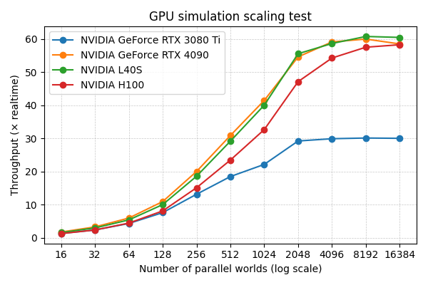
In practice, depending on the GPU model, maximum throughput is typically reached when between 2,000 and 17,000 worlds are simulated in parallel, as shown in the strong scaling test below. With a NVIDIA RTX 3080 Ti, the maximum throughput is ~30× realtime. On more powerful NVIDIA L40S and NVIDIA H100 GPUs, the maximum throughput is ~60× realtime. These results are obtained by running the benchmarking script in scripts/dev/run_gpu_benchmark.py, which performs the kinematic replay task described in this tutorial, but over 1000 steps instead of 500 for fairer comparison over sustained simulation.