Interacting with NeuroMechFly

Summary: In this tutorial, we will introduce the basic concepts of interacting with the simulated fly in a Markov Decision Process using the Gym interface. As a demonstration, we will replay experimentally recorded leg kinematics during walking in the simulator.

Markov Decision Process (MDP) and the Gym API

We formulated the control of NeuroMechFly as a partially observable Markov Decision Process (MDP). At each time step, the simulation provides the controller with an observation and, optionally, a user-defined reward. Then, the simulation receives an action from the controller and steps the physics forward accordingly. The observation space is a user-configurable subset of the state space including visual inputs, olfactory inputs, ground contacts, joint states (angles, angular velocities, and torques), and the position and velocity of the fly model within the arena. The action space includes the control signal (eg. angles for position control) for every actuated joint (eg. 7 degrees-of-freedom (DoFs) per leg * 6 legs) and the on/off signal for leg adhesion. This framework is easily extendable: the user can incorporate additional layers of sensory preprocessing or premotor computation into the MDP.

The biomechanical model and its interaction with the environment are encapsulated as a MDP task. A user-defined controller interfaces with the task through actions (red) and observations (blue). The user can extend the MDP task by adding preprogrammed processing routines for sensory inputs (purple) and motor outputs (light blue), to modify the action and observation spaces handled by the controller.

Our implementation of the partially observable MDP complies with the Gymnasium API. Gymnasium (a continuation of the now deprecated OpenAI Gym) is a package and standardized interface for developing and comparing control algorithms and benchmarking tasks. It provides a diverse collection of environments, ranging from classic control problems, Atari games, board games, and robotics simulations. Gym environments are designed to offer a common interface for controllers, in particular reinforcement learning agents, to interact with. This standardization makes it easier to develop and compare algorithms.

The overall steps for interacting with a Gym environment are:

1. Defining an environment

2. Reset the environment and get the initial observation

3. Interact with the environment with a loop:

   • Based on the last observation, the controller decides which actions to take

   • Step the simulation, applying the selected actions. The simulation will return you the new observation (and optionally some additional information)

   • Optional: render the simulation graphically

   • Break if certain conditions are met (eg. task is accomplished or failed), otherwise continue

4. Close the environment and analyze the results

This process is illustrated in the following code snippet:

env = MyEnvironement(...)
obs, info = env.reset()

for step in range(1000):    # let's simulate 1000 steps max
    action = ...    # your controller decides what to do based on obs
    obs, reward, terminated, truncated, info = env.step(action)
    env.render()
    if terminated or truncated:
        break

env.close()

Note that the action can be selected by any means defined by the user (eg. preprogrammed rules, algorithmic models, artificial neural networks).

The action and observation spaces

The action is a dictionary with the following keys and values:

• “joints”: The control signal for the actuated DoFs (eg. if NeuroMechFly.control == "position", then this is the target joint angle). This is a NumPy array of shape (|actuated_joints|,). The order of the DoFs is the same as NeuroMechFly.actuated_joints.

• “adhesion” (if sim_params.enable_adhesion is True): The on/off signal of leg adhesion as a NumPy array of shape (6,), one for each leg. The order of the legs is: LF, LM, LH, RF, RM, RH (L/R = left/right, F/M/H = front/middle/hind).

The observation is a dictionary with the following keys and values:

• “joints”: The joint states as a NumPy array of shape (3, |actuated_joints|). The three rows are the angle, angular velocity, and force at each DoF. The order of the DoFs is the same as NeuroMechFly.actuated_joints

• “fly”: The fly state as a NumPy array of shape (4, 3). 0th row: x, y, z position of the fly in arena. 1st row: x, y, z velocity of the fly in arena. 2nd row: orientation of fly around x, y, z axes. 3rd row: rate of change of fly orientation.

• “contact_forces”: Readings of the touch contact sensors, one placed for each of the body segments specified in NeuroMechFly.contact_sensor_placements. This is a NumPy array of shape (|contact_sensor_placements|, 3)

• “end_effectors”: The positions of the end effectors (most distal tarsus link) of the legs as a NumPy array of shape (6, 3). The order of the legs is: LF, LM, LH, RF, RM, RH (L/R = left/right, F/M/H = front/middle/hind).

• “fly_orientation”: NumPy array of shape (3,). This is the vector (x, y, z) pointing toward the direction that the fly is facing.

• “vision” (if sim_params.enable_vision is True): The light intensities sensed by the ommatidia on the compound eyes. This is a NumPy array of shape (2, num_ommatidia_per_eye, 2), where the zeroth dimension is the side (left, right in that order); the second dimension specifies the ommatidium, and the last column is for the spectral channel (yellow-type, pale-type in that order). Each ommatidium only has one channel with nonzero reading. The intensities are given on a [0, 1] scale.

• “odor_intensity” (if sim_params.enable_olfaction is True): The odor intensities sensed by the odor sensors (by default 2 antennae and 2 maxillary palps). This is a NumPy array of shape (odor_space_dimension, num_sensors).

terminated, truncated, and the info dictionary

In the Gym API, the step() method returns a terminated flag indicating whether the simulation has ended due to a condition under the MDP formulation (eg. task success/failure). The step() method also returns a truncated flag indicating whether the simulation has ended due to a condition outside the MDP formulation (eg. timeout). The provided NeuroMechFly environment always returns False for both terminated and truncated. The user can modify this behavior by extending the NeuroMechFly class.

Additionally, the step() method returns an info dictionary that contains arbitrary auxilliary information. The user can add any information to this dictionary by extending the NeuroMechFly class. The provided NeuroMechFly contains the following keys and values in the ``info`` dictionary:

• “raw_vision” (if sim_params.enable_vision and sim_params.render_raw_vision are both True): The eye camera rendering before it is transformed into ommatidia readings. This is a NumPy array of shape (2, nrows, ncols, 3) where the zeroth dimension is for the side (left, right in that order). The rest are the RGB image.

Example: Kinematic replay of experimentally recorded behavior

We now move on to an example where we kinematically replay some experimentally recorded walking behaviors. Specifically, we recorded a tethered fly walking on an air-suspended spherical treadmill using seven zoomed-in cameras from different angles. We then estimated the 3D positions of keypoints on the joints using DeepFly3D (Günel et al., Elife 2019) and used inverse kinematics to calculate the angle at each DoF. With these we will use a PD controller to actuate the DoFs of the simulated fly using these exact angles to see if the fly can walk untethered on flat terrain, as shown in the original NeuroMechFly paper (Lobato-Rios et al., Nature Methods 2022).

We start with the necessary imports:

import numpy as np
import pickle
import matplotlib.pyplot as plt
from pathlib import Path
from tqdm import trange

import flygym.common
import flygym.mujoco
import flygym.mujoco.preprogrammed

Let’s define some simulation parameters:

run_time = 1
sim_params = flygym.mujoco.Parameters(
    timestep=1e-4, render_mode="saved", render_playspeed=0.2, draw_contacts=True
)
actuated_joints = flygym.mujoco.preprogrammed.all_leg_dofs

We can now load recorded kinematics that are included with the FlyGym package:

data_path = flygym.common.get_data_path("flygym", "data")
with open(data_path / "behavior" / "210902_pr_fly1.pkl", "rb") as f:
    data = pickle.load(f)

The dataset is provided at 2000 Hz. We will try to run the simulation at \(\Delta t=0.0001s\) (10000 Hz), so let’s interpolate it 5x:

target_num_steps = int(run_time / sim_params.timestep)
data_block = np.zeros((len(actuated_joints), target_num_steps))
input_t = np.arange(len(data["joint_LFCoxa"])) * data["meta"]["timestep"]
output_t = np.arange(target_num_steps) * sim_params.timestep
for i, joint in enumerate(actuated_joints):
    data_block[i, :] = np.interp(output_t, input_t, data[joint])

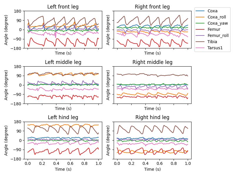
We can visualize the time series of DoF angles:

fig, axs = plt.subplots(
    3, 2, figsize=(8, 6), sharex=True, sharey=True, tight_layout=True
)
legs = [
    f"{side} {pos} leg"
    for pos in ["front", "middle", "hind"]
    for side in ["Left", "Right"]
]
for i, leg in enumerate(legs):
    ax = axs.flatten()[i]
    leg_code = f"{leg.split()[0][0]}{leg.split()[1][0]}".upper()
    for j, dof in enumerate(actuated_joints):
        if dof.split("_")[1][:2] != leg_code:
            continue
        ax.plot(output_t, np.rad2deg(data_block[j, :]), label=dof[8:])
    ax.set_ylim(-180, 180)
    ax.set_xlabel("Time (s)")
    ax.set_ylabel("Angle (degree)")
    ax.set_yticks([-180, -90, 0, 90, 180])
    ax.set_title(leg)
    if leg == "Right front leg":
        ax.legend(bbox_to_anchor=(1.04, 0.5), loc="center left", borderaxespad=0)
fig.savefig("outputs/kin_replay_joint_dof_time_series.png")

Now we can create a NeuroMechFly simulation instance and play out the recorded kinematics in the MDP loop:

nmf = flygym.mujoco.NeuroMechFly(
    sim_params=sim_params,
    init_pose="stretch",
    actuated_joints=actuated_joints,
    control="position",
)
obs, info = nmf.reset()
for i in trange(target_num_steps):
    # here, we simply use the recorded joint angles as the target joint angles
    joint_pos = data_block[:, i]
    action = {"joints": joint_pos}
    obs, reward, terminated, truncated, info = nmf.step(action)
    nmf.render()

100%|██████████| 10000/10000 [00:16<00:00, 608.34it/s]

To save the rendered video:

nmf.save_video("./outputs/kinematic_replay.mp4")

We can inspect the observation at the last step to see if they are consistent with our expectations:

for k, v in obs.items():
    print(f"{k}: shape {v.shape}")

joints: shape (3, 42)
fly: shape (4, 3)
contact_forces: shape (30, 3)
end_effectors: shape (6, 3)
fly_orientation: shape (3,)

The basic NeuroMechFly simulation always returns 0 as the reward. It always returns False for the terminated and truncated flags. The info is also empty. The user can extend the NeuroMechFly class to modify these behaviors.

print(f"reward: {reward}")
print(f"terminated: {terminated}")
print(f"truncated: {truncated}")
print(f"info: {info}")

reward: 0
terminated: False
truncated: False
info: {}